Stop Thieves And Mistakes! Protect Your Formulas Like A Sacred Territory In Google Sheets

APPS • DAILYTECH.ID - Safeguarding intellectual property or complex computations within shared spreadsheets requires effective cell protection. Google Sheets provides robust mechanisms to ensure that critical formulas remain untouched, preventing unauthorized editing while maintaining data integrity across collaborative teams.

To lock formulas in Google Sheets, use the “Protect sheets and ranges” feature found under the Data menu. Select the cell range containing your formulas, add a description, and set permissions to restrict editing only to specific users or prevent all non-owner edits, ensuring critical calculations remain tamper-proof across collaborators. Understanding these protection settings is crucial for any user needing to secure data models.

The Core Mechanism: How to Lock Formulas in Google Sheets

The process for how to lock formulas in google sheets centers entirely on the Protect sheets and ranges utility. This feature allows sophisticated control over granular areas of the spreadsheet, making it the definitive method for securing calculation outputs and preventing accidental corruption by collaborators. This is the essential procedure for anyone needing to how do i protect formulas in google sheets or how to lock all formulas in google sheets.

Identifying and Selecting the Formula Range

Effective protection begins with precise selection. Locking formulas requires isolating the cells that contain the complex calculations from the surrounding cells that are intended for user input.

1. Selection Strategy: Carefully highlight the cells, columns, or non-contiguous ranges that contain the formulas you intend to protect. For instance, if Column D is the result of a complex calculation based on inputs in Columns A, B, and C, you would select the entire range D2:D500 (or whichever rows are relevant).
2. Accessing the Protection Tool: Navigate to the main menu bar at the top of the Google Sheets interface.
   • Click the Data menu.
   • Select Protect sheets and ranges from the dropdown options.

This action opens a dedicated sidebar, usually titled “Protected sheets & ranges,” on the right side of your screen. This sidebar is where all security settings for your workbook are managed.

Applying Restrictions: Setting Permissions to Lock Formulas

Once the sidebar is open and you have clicked Add a sheet or range, you must define the scope of the protection and who is exempt from the restrictions. This step ensures you know how to protect cells in google sheets from editing.

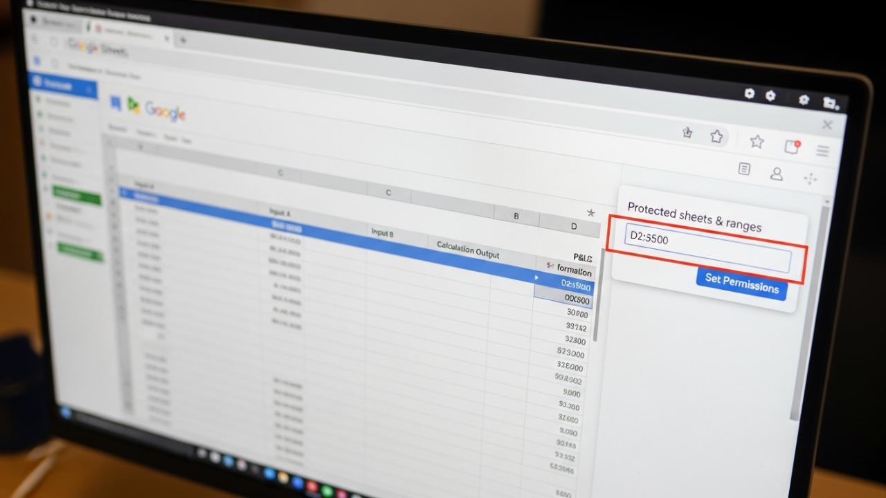
1. Verify the Range: Ensure the correct cell range is listed in the input field. If you selected the range beforehand, it should populate automatically. You may optionally add a descriptive name (e.g., “Monthly P&L Calculation”) for easy identification later.
2. Initiate Permissions Setting: Click the Set permissions button. A dialog box titled “Range editing permissions” will appear.
3. Choose the Restriction Type: You are presented with two primary options for security:
   • Show a warning when editing this range: This is a soft restriction, suitable for non-critical warnings where data integrity is important but not proprietary. Collaborators will see a pop-up warning but can still proceed with editing.
   • Restrict who can edit this range: This is the hard lock, required to truly secure formulas. Selecting this option triggers the user limitation settings.
4. Define Authorized Editors: If you chose to restrict editing, you must specify who retains the right to modify the content of the formulas:
   • Only you: This is the most secure setting, preventing all collaborators, regardless of their sheet access level, from editing the formulas.
   • Custom: Allows you to specify a list of email addresses (collaborators) who will be exempt from the lock. Note that the sheet owner is always authorized to edit protected ranges.
   • Domain: If operating within a corporate Google Workspace environment, you might restrict editing to users within a specific organizational domain.
5. Finalizing the Lock: Click Done or Save to apply the security settings. The formulas within the specified range are now locked and cannot be accidentally or intentionally overwritten by unauthorized parties.

Granular Control: Locking Specific Cells and Ranges

The strength of the Google Sheets protection tool lies in its flexibility, allowing users to lock formulas in google sheets without disrupting general data entry.

Protecting Formulas Without Locking the Entire Sheet

A common requirement for collaborative project managers is how to protect cells in google sheets without protecting sheet. The Protect sheets and ranges feature is specifically designed for this purpose. Unlike the sheet protection option (which locks every cell on a tab), range protection allows users to define multiple, non-contiguous protected zones within a single sheet.

Scenario Example: A project tracker sheet has 10 columns. Columns A-C are input fields (unlocked). Column D contains the formula for Status (locked). Columns E-J are also input fields (unlocked).

To achieve this, the user simply follows the core protection method but specifies only the range D2:D500. All cells outside of this specific range remain fully editable by all collaborators. This technique is highly effective for maintaining the integrity of calculated data models while promoting seamless team collaboration.

How to Lock Certain Cells in Google Sheets Individually

If only a handful of isolated cells contain complex formulas—for example, summary metrics in B1, E10, and G25—the protection can be applied to these cells individually. While seemingly inefficient to define three separate protections for single cells, this is the correct technical approach.

1. Access the protection sidebar.
2. Add a new range: B1:B1. Set permissions.
3. Add another range: E10:E10. Set permissions.
4. Add a final range: G25:G25. Set permissions.

This demonstrates that protection in Google Sheets scales from single cells up to large, contiguous ranges, providing maximum control over intellectual property.

Advanced Security: Hiding Formulas and Handling Partial Locks

For intellectual property protection, such as proprietary pricing algorithms or complex data transformations, users often need to not only lock the formula but also obscure the underlying logic.

How to Lock and Hide Formulas in Google Sheets

Google Sheets, unlike desktop Excel, does not possess a native “hidden” attribute that masks the formula text in the formula bar while leaving the cell protected. Therefore, achieving true intellectual property security when sharing highly sensitive calculations requires a layered approach:

1. Locking the Cell (Essential): First, the cell must be locked using the Protect sheets and ranges method with the most restrictive permissions (Only you). This prevents unauthorized users from double-clicking the cell and changing the formula.
2. Restricting Viewing Access (Supplementary): If the formula logic itself must be obscured from view, the only method is to restrict viewing access to the document entirely, or move the proprietary calculation logic to a hidden sheet and ensure the sheet tab itself is protected (locked). If a user can view the sheet, they can typically view the formula bar content in a protected range, even if they cannot edit it.
3. Using Google Apps Script: The most robust method involves having the formulas live inside Google Apps Script (GAS). The calculation results are then pushed back to the sheet cells as static values rather than active formulas. This way, the proprietary logic is contained within the backend code, which collaborators cannot access, and the output cells can be further protected as static data.

Addressing Partial and Conditional Protection

Users often ask how to lock part of a formula in google sheets. It is critical to understand that protection is always applied to the cell as a container. You cannot lock the SUM(A1:A5) portion of a formula while leaving the +100 portion editable.

Instead, advanced users must manage protection by function:

• Input Management: Ensure all cells referenced by the formula (the input data) remain unlocked so collaborators can update the variables.
• Output Management: Ensure the cell containing the calculated result (the locked formula) is protected.

Achieving Conditional Locking with Script

Google Sheets does not natively support how to conditionally lock cells in google sheets (e.g., automatically lock a row once a “Status” cell is marked “Complete”). This functionality requires Google Apps Script.

A script can be written to monitor sheet activity (e.g., onEdit). When a trigger condition is met (e.g., cell C5 is changed to “Approved”), the script automatically executes code that programmatically applies range protection to the corresponding row of formulas, dynamically locking the data based on user input. This requires intermediate coding skill but provides the highest level of automation for data management.

Protecting Formulas Across Different Platforms

The core steps for how to lock formulas in google sheets are universally applied, but the interface nuances differ slightly when transitioning from desktop to mobile environments.

Mobile Protection: How to Lock Cells in Google Sheets App

For users collaborating via mobile devices (iOS or Android), protection must be configured using the mobile application interface. The functionality for how to lock cells in google sheets mobile mirrors the desktop tool.

1. Accessing the Menu: Open the Google Sheets app and navigate to the desired sheet.
2. Select Range: Tap and hold the screen to select the range of cells containing the formulas.
3. Protection Interface: Look for the More Options icon, typically represented by three vertical dots (⋮) in the top-right corner, or a menu button on Android.
4. Protect Range: Select Protect range from the resulting menu options.
5. Set Permissions: The app will present the familiar permissions dialog, allowing you to restrict editing to specific users or solely yourself, just like the desktop version.

Whether using how to lock cells in google sheets android or iOS, the security principles and restriction options remain identical.

Desktop Interfaces: Mac and PC Consistency

Users asking how to lock formula in google sheets mac will find the process identical to the standard PC desktop instructions. The interface, menus (Data > Protect sheets and ranges), and permissions dialogs are unified across Chrome, Safari, and other browsers on both macOS and Windows operating systems. There are no specialized Mac commands required for this protection feature.

Clarification: Protection vs. Reference Locking

A fundamental confusion arises when users mix up security protection with formula stability. This distinction is crucial for intermediate users learning how to lock reference cells in google sheets.

The Functional Lock: Using the Dollar Sign ($)

The dollar sign ($) is used within a formula to create an absolute cell reference. This is a functional feature of spreadsheet software, not a security mechanism.

Example:

• A relative reference: =A1 (Changes to =A2 when dragged down one row).
• An absolute reference: =$A$1 (Remains =$A$1 no matter where the formula is dragged or copied).

The dollar sign dictates how the formula behaves when it is moved. If a user inputs =$A$1, they are using how to lock cells in google sheets dollar sign to stabilize the reference point. However, any unauthorized collaborator can still delete the formula entirely and type “Hello” in the cell, regardless of the dollar signs used within the formula text.

Summary of Differences

Feature	Purpose	Location	Security Implication
Cell Protection	Prevents users from modifying, deleting, or overwriting the cell content (formula or data).	Data Menu > Protect sheets and ranges	High (Security)
Absolute Referencing	Ensures the formula’s reference coordinates (e.g., A1) do not shift when the formula is copied or moved.	Within the Formula Bar ($ symbol)	None (Functional)

To truly secure critical formulas, users must employ Cell Protection. Absolute referencing is necessary to ensure the calculation itself works correctly across a range, but it offers zero defense against malicious or accidental user edits.

Managing and Reviewing Protection Settings

Over time, team compositions change, and security requirements evolve. Effective project management includes regular review of protection settings to ensure accessibility remains appropriate and security protocols are not bypassed.

Reviewing Existing Locks

All existing range and sheet protections are managed through the protection sidebar:

1. Navigate to Data > Protect sheets and ranges.
2. The sidebar lists every protected range, along with the name/description you provided.
3. Clicking on any listed protection highlights the corresponding range on the spreadsheet and allows you to modify the permissions or delete the protection entirely.

Modifying and Removing Protection

To remove a formula lock or change the list of authorized editors:

1. Select the relevant protected range in the sidebar.
2. Click Change permissions.
3. Adjust the restricted list or switch the restriction level (e.g., changing from “Only you” to “Custom”).
4. If the protection is no longer needed, click the trash can icon (Remove protection) and confirm the action.

Maintaining a secure collaborative environment requires both setting the initial lock and actively managing the permissions list as the project progresses. Utilizing the range protection feature rigorously ensures critical data calculations remain intact, establishing a reliable data integrity foundation for all analysis derived from the Google Sheet.

FAQs – Lock Formulas In Google Sheets